Chapter 1 Radioactivity

1.1 Units

Before we begin, a quick note on units:

1. Nuclear sizes are typically of order ${10}^{-15}\mathrm{m}$ (1 fm).

2. Nuclear time scales have a vast range, e.g. half-life can range from ${10}^{-20}\mathrm{s}$ to greater than the age of the Universe!

3. Nuclear energies are typically measured in MeV, where $1\mathrm{eV}=1.602\times {10}^{-19}\mathrm{J}$.

4. Nuclear masses are typically measured in the unified atomic mass unit (u), defined such that the mass of a Carbon-12 atom = 12 u. In terms of SI units, $1\mathrm{u}=1.66054\times {10}^{-27}\mathrm{kg}$.

   A Carbon-12 nucleus has 6 protons and 6 neutrons. Nucleons therefore have a mass of around 1 u (since the mass of the electron is much smaller than the mass of the proton and neutron, and the mass of protons/neutrons are approximately the same), where $1\mathrm{u}=931.5\mathrm{MeV}/{\mathrm{c}}^2$. Note I have now defined the mass in terms of energy divided by $c^2$, using the fact that $E=m{c}^2$. This is useful as we will commonly multiply masses by $c^2$ to obtain the energy, and the factors of $c$ will therefore cancel.

   As an example, the proton has a mass of $m_p=1.673\times {10}^{-27}\mathrm{kg}$ in SI units. This is equal to $m_p=938.3\mathrm{MeV}/{\mathrm{c}}^2$. The neutron has a mass of $m_n=1.675\times {10}^{-27}\mathrm{kg}$ in SI units. This is equal to $m_n=940.6\mathrm{MeV}/{\mathrm{c}}^2$.

Working in these units will make calculations easier and will be less likely to lead to mistakes.

1.2 Radioactive decay

The nucleus consists of protons (positively charged) and neutrons (neutral), which have approximately the same mass (the mass difference is important however in calculations!). Isotopes are defined as having different numbers of neutrons. Deuterium, for example (whose nucleus consists of 1 proton and 1 neutron), is an isotope of hydrogen.

Definition 1.2.1 (Radioactive Decay).

The spontaneous emission of radiation that changes the state of the nucleus.

Definition 1.2.2 (Nuclear notation).

We will define a nucleus by

$${}_Z{}^A\mathrm{X},$$ (1.1)

where $Z$ is the proton number (also called the atomic number) and $A=Z+N$ is the mass number, where $N$ is the number of neutrons. $X$ is the name of the nucleus, and is unique for a given $Z$. The $Z$ number is therefore sometimes omitted for common nuclei.

Radioactivity was discovered in 1896 by Henri Becquerel when he realised that Uranium was darkening a photographic plate in a cupboard. The Curies discovered more radioactive materials and realised there were three types of decay:

Alpha decay ($\alpha$)

A helium nucleus (2 protons and 2 neutrons) is emitted from a parent nucleus. It is strongly ionising, heavy (compared to the other types of radioactive decay), and has a charge of $+2e$. It is very damaging if inside the body.

Beta decay ($\beta$)

A high energy electron or positron (the anti-particle of an electron) is emitted from the nucleus. In the case of an electron being emitted (sometimes called ${\beta }^{-}$ decay), a neutron in the parent nucleus decays into a proton and an electron (plus an electron anti-neutrino). It is less ionising than $\alpha$ decay, but has a much faster speed, with lower charge ($-e$ for an electron or $+e$ for a positron). In the case of a positron being emitted (sometimes called ${\beta }^{+}$ decay), a proton in the parent nucleus decays into a neutron and a positron (plus an electron neutrino).

Gamma decay ($\gamma$)

The nucleus de-excites and emits a gamma ray photon (like electron transitions leading to photons in atoms). It is very energetic, interacts weakly with matter, and is uncharged.

Figure 1.1: Segre chart showing neutron number $N$ versus proton number $Z$ for known nuclides. Stable nuclei (shown in black) form a narrow valley of stability. The chart also indicates the dominant decay mode for unstable nuclei in different regions.

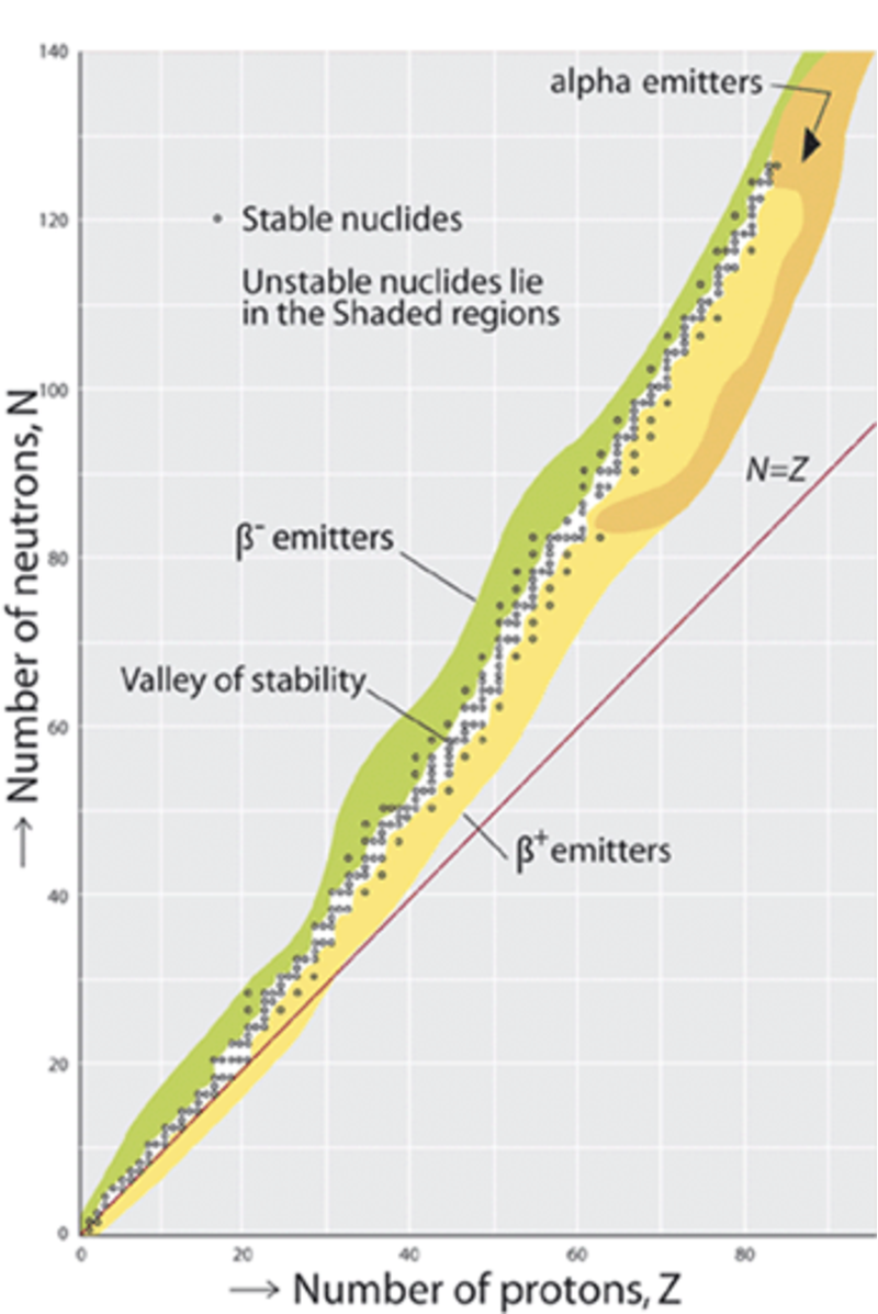
We will discuss each of these in more detail shortly. Of about 2500 known nuclides, only about 300 are stable. The stable nuclei form a narrow distribution on a plot of $N$ versus $Z$, as shown in Fig. 1.1. This plot is known as a Segre chart. The stability valley moves away from the $N=Z$ line for large $Z$. Larger nuclei need more neutrons relative to protons to remain stable, since neutrons are uncharged and have no repulsive Coulomb forces.

Nuclei can decay by either alpha or beta emission to move from the unstable regions towards the stable valley. To move on this diagram they must change $N$ or $Z$ or both. Heavier nuclei tend to decay by $\alpha$ decay, and lighter nuclei tend to decay by beta emission (those with a neutron excess decay by ${\beta }^{-}$ emission and those with a proton excess by ${\beta }^{+}$ emission). No nuclide with $A>209$ or $Z>83$ (Bismuth, Bi) is stable.

1.3 Natural radioactivity

The earth formed about $4.5\times {10}^9$ years ago from the debris of long dead stars. Most of the elements were radioactive but have since decayed into stable nuclei. However, a few have half-lives long compared to the age of the earth and so we can still observe their radioactivity. Most are very heavy elements. They decay by $\alpha$ and $\beta$ emission. $\alpha$ emission decreases $A$ by 4, whereas $\beta$ emission leaves $A$ unchanged. There are therefore 4 independent decay chains, as shown in Tab. 1.1. The decay process will concentrate the nuclei in the longest-lived member of the chain, and provided its half-life is of the order of the age of the earth (or longer), we can still observe that activity today.

			Longest-Lived Member
Name of Series	Type	Final Nucleus (Stable)	Nucleus	Half-Life (y)
Thorium	4n	208Pb	232Th	$1.41\times {10}^{10}$
Neptunium	4n+1	209Bi	237Np	$2.14\times {10}^6$
Uranium	4n+2	206Pb	238U	$4.47\times {10}^9$
Actinium	4n+3	207Pb	235U	$7.04\times {10}^8$

Table 1.1: The disintegration series of the heavy elements ($n$ is an integer).

If it were not for the very long half-life of ²³⁵U and ²³⁸U there would be no natural uranium and so no obvious source of nuclear power.

1.4 Activity

Definition 1.4.1 (Activity).

Defined as the number of decays per second.

The S.I. unit of activity is the Becquerel (Bq), where 1 Bq = 1 decay/s. However an older unit is still in regular use, the Curie (Ci), originally defined as the activity of 1 g of radium. 1 Ci = $3.7\times {10}^{10}$ Bq.

1.5 Radioactive decay law

The number of radioactive nuclei, $dN$, decaying in a time $dt$ is proportional to $N$, so

$$\frac{dN}{dt}=-\lambda N,$$ (1.2)

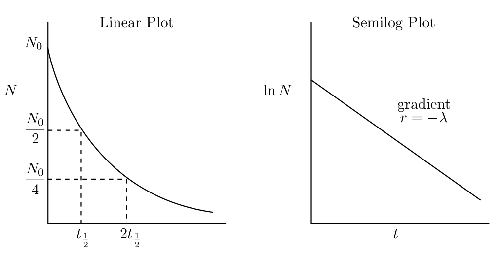
where $\lambda$ is the disintegration or decay constant, which has units of inverse time. Eqn. 1.2 can be integrated to give the exponential law of radioactive decay

$$N=N_0{e}^{-\lambda t},$$ (1.3)

where $N_0$ is the number of nuclei at $t=0$. The half-life, $t_{1/2}$, is the time taken for half of the material to decay. Putting $N=N_0/2$ in Eqn. 1.3 gives

${\displaystyle \frac{N_0}{2}}$ $=$ $N_0{e}^{-\lambda t_{1/2}},$ (1.4)

$t_{1/2}$ $=$ ${\displaystyle \frac{\ln 2}{\lambda }}.$

These decay laws are shown in Fig. 1.2.

Figure 1.2: Exponential law of radioactive decay.

Example 1.5.1 (Carbon Dating).

Primary cosmic radiation converts ¹⁴N in the atmosphere into ¹⁴C, which has a half-life of 5730 years. This combines with oxygen to form ${\mathrm{CO}}_2$ which is taken up by plants. When the plant dies the decay of the ¹⁴C radioactivity can be used to determine its age. If the activity of a sample of wood found in the tomb of one of the Pharaohs is 6.8 counts/min/gram of carbon and the activity of ¹⁴C in living plant material is 15.3 counts/min/gram of carbon, what is the age of the wood sample?

Solution.

The activity of the sample is given by

$$A=\lambda N,$$ (1.5)

so follows the same decay law as the number of nuclei, $A=A_0{e}^{-\lambda t}$. Rearranging gives

$t$ $=$ ${\displaystyle \frac{\ln (A_0/A)}{\lambda }},$

$t$ $=$ $t_{1/2}{\displaystyle \frac{\ln (A_0/A)}{\ln 2}},$

$t$ $=$ $6704\mathrm{years}.$

∎

It is also useful to consider the mean lifetime, $\tau$, defined as the average time a nucleus is likely to survive before it decays. This is given by

$$\tau =\frac{{\int }_0^{\mathrm{\infty }}t|dN/dt|𝑑t}{{\int }_0^{\mathrm{\infty }}|dN/dt|𝑑t}.$$ (1.6)

After integrating by parts and performing some algebra, one finds

$$\tau =\frac{1}{\lambda }.$$ (1.7)

Activity is the rate at which decays occur, i.e.

$$A=\lambda N.$$ (1.8)

1.5.1 Decay sequences

As discussed, nuclei often decay in sequence. Consider the decay sequence of 3 nuclei:

$$A\stackrel{{\lambda }_A}{\to }B\stackrel{{\lambda }_B}{\to }C$$ (1.9)

where nuclide $A$ is the first in the chain, and nuclide $C$ is stable. The notation means nuclide $A$ will decay with decay constant ${\lambda }_A$, and nuclide $B$ will decay with decay constant ${\lambda }_B$. The differential equations describing the system are

${\displaystyle \frac{d{N}_A}{dt}}$ $=$ $-{\lambda }_A{N}_A,$ (1.10)

${\displaystyle \frac{d{N}_B}{dt}}$ $=$ ${\lambda }_A{N}_A-{\lambda }_B{N}_B,$ (1.11)

${\displaystyle \frac{d{N}_C}{dt}}$ $=$ ${\lambda }_B{N}_B.$ (1.12)

The difference here is that nuclide $B$ is also being produced at a rate of ${\lambda }_A{N}_A$ in time $dt$, i.e. at the same rate at which nuclide $A$ is decaying. This intuitively makes sense, as nuclide $A$ is decaying to $B$. Similarly, nuclide $C$ is being produced at a rate of ${\lambda }_B{N}_B$ in time $dt$. We will solve for such a decay sequence in the examples. Note that this treatment can be generalized to longer decay chains of nuclei.

Example 1.5.2 (Decay Sequence).

In a decay sequence, the nucleus $N_1$ decays to $N_2$ with a decay constant ${\lambda }_1$. The nucleus $N_2$ subsequently decays with a decay constant ${\lambda }_2$. Assuming only $N_1$ is present at $t=0$, calculate $N_1(t)$ and $N_2(t)$.

Solution.

The rate equations are

${\displaystyle \frac{d{N}_1}{dt}}$ $=$ $-{\lambda }_1{N}_1,$

${\displaystyle \frac{d{N}_2}{dt}}$ $=$ ${\lambda }_1{N}_1-{\lambda }_2{N}_2.$

The solution to the first equation is $N_1(t)=N_1(0)e^{-{\lambda }_{1}t}$. To solve the second

${\displaystyle \frac{d{N}_2}{dt}}+{\lambda }_2{N}_2$ $=$ ${\lambda }_1{N}_1.$

Multiplying both sides by $e^{{\lambda }_{2}t}$ gives

$e^{{\lambda }_{2}t}{\displaystyle \frac{d{N}_2}{dt}}+{\lambda }_2{e}^{{\lambda }_{2}t}{N}_2$ $=$ ${\lambda }_1{N}_1{e}^{{\lambda }_{2}t},$

${\displaystyle \frac{d\left(e^{{\lambda }_{2}t}{N}_2\right)}{dt}}$ $=$ ${\lambda }_1{N}_1{e}^{{\lambda }_{2}t}={\lambda }_1{N}_1(0)e^{({\lambda }_2-{\lambda }_1)t}.$

Integrating both sides gives

$e^{{\lambda }_{2}t}{N}_2$ $=$ ${\displaystyle \frac{{\lambda }_1{N}_1(0)}{{\lambda }_2-{\lambda }_1}}{e}^{({\lambda }_2-{\lambda }_1)t}+C.$

Applying the initial condition $N_2(0)=0$ gives $C=-\frac{{\lambda }_1{N}_1(0)}{{\lambda }_2-{\lambda }_1}$, hence

$e^{{\lambda }_{2}t}{N}_2$ $=$ ${\displaystyle \frac{{\lambda }_1{N}_1(0)}{{\lambda }_2-{\lambda }_1}}\left(e^{({\lambda }_2-{\lambda }_1)t}-1\right),$

$N_2(t)$ $=$ ${\displaystyle \frac{{\lambda }_1{N}_1(0)}{{\lambda }_2-{\lambda }_1}}\left(e^{-{\lambda }_{1}t}-e^{-{\lambda }_{2}t}\right).$

∎

1.6 Types of decay

The three principal decay types are $\alpha ,\beta ,\gamma$. In $\alpha$ and $\beta$ decay processes an unstable nucleus emits a particle as it tries to become more stable. In $\gamma$ decay an excited nuclear state decays toward the ground state without changing the nuclear species.

1.6.1 $\alpha$ decay

In this process a ${}_2{}^{}{}_{}{}^4$He nucleus ($\alpha$ particle) is emitted from the parent nucleus

$${}_Z{}^A\mathrm{X}{\to }_{Z-2}^{A-4}\mathrm{Y}{+}_2^4\mathrm{He}.$$ (1.13)

An example is the decay of radium

$${}_{88}{}^{226}\mathrm{Ra}{\to }_{86}^{222}\mathrm{Rn}{+}_2^4\mathrm{He},$$ (1.14)

with $t_{1/2}=1600$ years and an $\alpha$ particle KE of 4.8 MeV. In order to calculate the energy release, $Q$, we can use a general equation that we will use frequently throughout the module. Due to the conservation of energy and momentum, the $\alpha$ particle carries around $98\%$ of the $Q$ value, with the much heavier daughter nuclear nucleus carrying only about $2\%$.

Definition 1.6.1 (Energy release).

To calculate the energy release, $Q$, of a decay we consider the difference in nuclear mass between reactants and products, and multiply by $c^2$:

$$Q=\left[\sum M_{\mathrm{N},\mathrm{reactants}}-\sum M_{\mathrm{N},\mathrm{products}}\right]c^2.$$ (1.15)

Note that the masses are nuclear masses (denoted by a subscript N), as opposed to atomic masses. This is because these are nuclear reactions, involving the decay of the nucleus.

For a decay to be energetically possible we require $Q>0$. Note, however, that this doesn’t necessarily mean the decay will occur spontaneously. In nuclear fission, for example, there is also a large potential barrier to overcome, which requires fission to be induced.

Careful 1.6.1.

We will primarily be interested in nuclear masses. If you are given atomic masses (denoted by a subscript A) you can convert to nuclear mass by

$$M_N=M_A-Z{m}_{\mathrm{e}},$$ (1.16)

where $m_{\mathrm{e}}$ is the electron mass. I will emphasise this point several times as it’s an easy thing to slip up on!

Alpha emission is a Coulomb repulsion effect and becomes more significant for heavy nuclei because the Coulomb force increases as $Z^2$, whereas the nuclear binding force increases with $A$ (see later). Why is it always an alpha particle that is ejected? For the decay of ²³²U we can calculate the energy release for different particles. We require $Q>0$, which is only possible for the $\alpha$ particle, as shown in Tab. 1.2.

Example 1.6.1 (Energy Release).

Question: Calculate the energy release by the decay

$${}_{92}{}^{232}\mathrm{U}{\to }_{90}^{228}\mathrm{Th}{+}_2^4\mathrm{He}.$$ (1.17)

The atomic masses of ${}_{92}{}^{232}\mathrm{U}$, ${}_{90}{}^{228}\mathrm{Th}$ and ${}_2{}^4\mathrm{He}$ are $232.03716\mathrm{u}$, $228.02874\mathrm{u}$ and $4.00260\mathrm{u}$ respectively, where $1\mathrm{u}=931.5\mathrm{MeV}/{\mathrm{c}}^2$. The mass of the electron is $0.511\mathrm{MeV}/{\mathrm{c}}^2$.

Solution.

$$Q=\left[\sum M_{\mathrm{N},\mathrm{reactants}}-\sum M_{\mathrm{N},\mathrm{products}}\right]c^2.$$ (1.18)

$Q$ $=$ $[M_{\mathrm{N}}{(}_{92}^{232}\mathrm{U})-M_{\mathrm{N}}{(}_{90}^{228}\mathrm{Th})-M_{\mathrm{N}}{(}_2^4\mathrm{He})]c^2.$ (1.19)

$=$ $[M_{\mathrm{A}}{(}_{92}^{232}\mathrm{U})-92m_e-M_{\mathrm{A}}{(}_{90}^{228}\mathrm{Th})+90m_e-M_{\mathrm{A}}{(}_2^4\mathrm{He})+2m_e]c^2.$ (1.20)

$=$ $[M_{\mathrm{A}}{(}_{92}^{232}\mathrm{U})-M_{\mathrm{A}}{(}_{90}^{228}\mathrm{Th})-M_{\mathrm{A}}{(}_2^4\mathrm{He})]c^2,$ (1.21)

$=$ $\left[232.03716-228.02874-4.00260\right]\times 931.5\mathrm{MeV},$ (1.22)

$=$ $5.4\mathrm{MeV}.$ (1.23)

This is fairly typical for $\alpha$ decay. ∎

Emitted Particle	Energy Release (MeV)
n	-7.26
1H	-6.12
2H	-10.70
3H	-10.24
3He	-9.92
4He	+5.41
5He	-2.59
6He	-6.19
6Li	-3.79
7Li	-1.94

Table 1.2: Energy release for different decay modes of ²³²U.

Figure 1.3: The inverse relationship between $\alpha$ decay half-life and decay energy.

Geiger-Nuttall rule

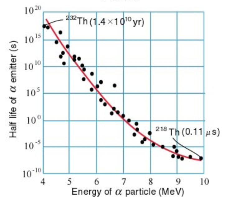
There is a strong relationship (the Geiger-Nuttall rule) relating the energies of the emitted alpha particle and the half-lives of the nuclides, with large energies associated with short half-lives. The variation in half-life is astounding (note the log axis in Fig. 1.3). For example, ²³²Th has $t_{1/2}=1.4\times {10}^{10}$ years and $Q=4.08$ MeV, while ²¹⁸Th has $t_{1/2}=1.0\times {10}^{-7}$ s and $Q=9.85$ MeV.

The Geiger-Nuttall rule can largely be explained by a model based on quantum mechanical tunneling (Gamow, Gurney and Condon in 1928). In this theory, an $\alpha$ particle is pre-formed inside a nucleus. There is actually not much reason to believe that $\alpha$ particles exist separately inside the nucleus, but nevertheless, the model works quite well.

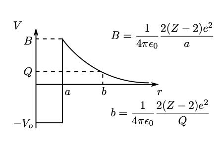
The $\alpha$ particle moves in the spherical potential well, $V(r)$, created by the daughter nucleus. This is shown in Fig. 1.4, where $r$ represents the distance between the $\alpha$ particle and daughter nucleus. The $\alpha$ particle has an energy equal to $Q$, since almost all of the energy released is carried by it. There are three regions of interest:

1. In the region , the potential well has a depth $-V_0$. The $\alpha$ particle is classically confined to this region.

2. Outside of this region, there is a (repulsive) Coulomb potential, which cuts off at a radius $r=a$. For , there is a barrier region, where the potential energy is greater than $Q$.

3. The region $r>b$ is classically permitted outside the barrier.

From a classical point of view, the $\alpha$ particle in the potential well would sharply reverse its motion every time it tried to pass $r=a$. Quantum mechanically, however, there is a chance of tunneling to the classically permitted region outside the barrier.

Careful 1.6.2.

The Coulomb potential energy between two nuclei with charges $Q_1=Z_{1}e$ and $Q_2=Z_{2}e$ at a distance $r$ is given by

$$V=\frac{Q_1{Q}_2}{4\pi {ϵ}_{0}r}=\frac{Z_1{Z}_2{e}^2}{4\pi {ϵ}_{0}r}.$$ (1.24)

Be careful to include the $Z_1$ and $Z_2$ factors, and remember it has a $1/r$ dependence.

Figure 1.4: Potential energy diagram for an $\alpha$ particle/daughter nucleus system.

To obtain the tunnelling probability recall the time-independent Schrödinger equation for a particle of mass $m$ in one dimension,

$$-\frac{{\mathrm{\hslash }}^2}{2m}\frac{d^2\psi }{d{x}^2}+V(x)\psi (x)=E\psi (x),$$ (1.25)

where $\psi (x)$ is the wave function. The complete solution, including time dependence is $\mathrm{\Psi }(x,t)=\psi (x)e^{-iEt/\mathrm{\hslash }}$.

For the case of $E>V(x)$ the solutions for $\psi (x)$ are oscillatory. Assuming a constant potential $V(x)=V_c$, we can attempt a trial solution of the form

$$\psi =A{e}^{i{k}_{1}x}+\tilde{B}{e}^{-i{k}_{1}x}.$$ (1.26)

Note I have used $\tilde{B}$ here to avoid confusion with the $B$ in Fig. 1.4. Plugging this into Eqn. 1.25 gives the constant $k_1$,

$$k_1=\sqrt{\frac{2m(E-V_c)}{{\mathrm{\hslash }}^2}}.$$ (1.27)

The solutions are exponential when . Assuming a constant potential $V(x)=V_c$, we can attempt a trial solution of the form

$$\psi =C{e}^{k_{2}x}+D{e}^{-k_{2}x}.$$ (1.28)

Plugging this into Eqn. 1.25 gives the constant $k_2$,

$$k_2=\sqrt{\frac{2m(V_c-E)}{{\mathrm{\hslash }}^2}}.$$ (1.29)

The unknown coefficients $A,\tilde{B},C,D$ can be found by applying continuity conditions and normalization of the wavefunction. We will perform this calculation when considering the nuclear potential of the deuteron later in the semester.

Figure 1.5: Simplified potential.

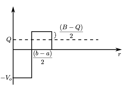
Unfortunately, our model for the nuclear potential is not constant. However, we can simplify the potential that the $\alpha$ particle has to tunnel through to that of Fig. 1.5. The average value of $V_c-E$ in the barrier region is $(B-Q)/2$, which means (in the barrier region)

$$k_2=\sqrt{\frac{m(B-Q)}{{\mathrm{\hslash }}^2}}.$$ (1.30)

Obtaining solutions in the other regions and applying boundary conditions, one can compute the transmission coefficient, $P$, defined as the probability of a particle tunneling through a barrier (see the Krane textbook for further details),

$$P\approx e^{-k_2(b-a)}.$$ (1.31)

The decay constant is given by

$$\lambda =fP,$$ (1.32)

where $f$ is the frequency with which the $\alpha$ particle hits the barrier, roughly $v/a$, where $v$ is the velocity of the $\alpha$ particle.

Example 1.6.2 (Radioactivity).

Question: For a typical heavy nucleus with $Z=90$, $a=7.5$ fm, and an $\alpha$ particle energy of 6 MeV, estimate $t_{1/2}$. You may assume $f=6.1\times {10}^{21}$ Hz.

Solution.

Solution: First, work out the barrier height. A useful quantity is

$$\frac{e^2}{4\pi {ϵ}_0}=1.440\mathrm{MeV}\mathrm{fm}.$$ (1.33)

Therefore

$$B=\frac{2(90-2)\times 1.440}{7.5}\mathrm{MeV}=33.8\mathrm{MeV}.$$ (1.34)

The distance $b$ is when the particle energy is equal to the Coulomb potential energy,

$$b=\frac{2(90-2)\times 1.440}{6}\mathrm{fm}=42.2\mathrm{fm}.$$ (1.35)

We can now compute $k$. The $\alpha$ particle has a mass of $4.00$u. $1\mathrm{u}=931.5\mathrm{MeV}/c^2$, so $m=3.726\times {10}^3\mathrm{MeV}/c^2$. Using the relation $\mathrm{\hslash }c=197.3\mathrm{MeV}\mathrm{fm}$ then

$k$ $=\sqrt{{\displaystyle \frac{3.726\times {10}^3(33.8-6)}{{197.3}^2}}}{\mathrm{fm}}^{-1}$ (1.36)

$=1.63{\mathrm{fm}}^{-1}.$

We can then calculate

$$P\approx e^{-1.63\times (42.2-7.5)}\approx 2.7\times {10}^{-25}.$$ (1.37)

Finally $\lambda \approx 6.1\times {10}^{21}\times 2.7\times {10}^{-25}\approx 1.7\times {10}^{-3}{\mathrm{s}}^{-1}$. This gives $t_{1/2}\approx 400$ s. We can do the same calculation changing $Q$ to 5 MeV to find $P\approx 1\times {10}^{-30}$, so $t_{1/2}\sim {10}^8$ s! ∎

1.7 $\beta$ decay

$\beta$ decay is the process by which a nuclide can correct a proton or a neutron excess through

$n$ $\to$ $p+e^{-}+{\overline{\nu }}_{\mathrm{e}}{\beta }^{-}\mathrm{decay},$ (1.38)

$p$ $\to$ $n+e^{+}+{\nu }_{\mathrm{e}}{\beta }^{+}\mathrm{decay},$

$p+e^{-}$ $\to$ $n+{\nu }_{\mathrm{e}}\mathrm{orbital}\mathrm{electron}\mathrm{capture}.$

The positron ($e^{+}$) is the anti-particle of an electron. It has the same mass but equal and opposite charge.

Careful 1.7.1.

Note that a single proton is stable as , leading to . This decay can occur inside a nucleus though, since when we compute the $Q$ value for $\beta$ decay we use the full nuclear equation.

Pauli proposed in 1931 that an unknown particle was released in the decay process. These were later named by Fermi as the neutrino, $\nu$, and anti-neutrino, $\overline{\nu }$. Note that here we have labeled the neutrinos as electron neutrinos, since there are other types of neutrino (see later).

The corresponding nuclear equations are therefore

${}_Z{}^A\mathrm{X}$ $\to$ ${}_{Z+1}{}^A\mathrm{Y}+e^{-}+{\overline{\nu }}_{\mathrm{e}}{\beta }^{-}\mathrm{decay}$

${}_Z{}^A\mathrm{X}$ $\to$ ${}_{Z-1}{}^A\mathrm{Y}+e^{+}+{\nu }_{\mathrm{e}}{\beta }^{+}\mathrm{decay}$

${}_Z{}^A\mathrm{X}+e^{-}$ $\to$ ${}_{Z-1}{}^A\mathrm{Y}+{\nu }_{\mathrm{e}}\mathrm{OEC}.$ (1.39)

In the case of $\alpha$ decay, the $\alpha$ particles are emitted with precise energies, but for $\beta$ decay there is a continuous distribution up to a maximum energy. For example, in the case of ²¹⁰Bi, the change in the nuclear mass suggests that the $\beta$ particles should have an energy of 1.16 MeV. Instead, a continuous distribution is observed, as shown in Fig. 1.6. This is due to the neutrino sharing some of the kinetic energy.

Careful 1.7.2.

Make sure that appropriate quantities in equations like 1.7 are conserved. You already know that energy, momentum, and charge should be conserved. Later we will discuss other conserved quantities.

Figure 1.6: Electron energy distribution from the $\beta$ decay of ²¹⁰Bi.

Examples of $\beta$ decay include

${}_6{}^{14}\mathrm{C}$ $\to$ ${}_7{}^{14}\mathrm{N}+e^{-}+{\overline{\nu }}_{\mathrm{e}},$ (1.40)

${}_9{}^{18}\mathrm{F}$ $\to$ ${}_8{}^{18}\mathrm{O}+e^{+}+{\nu }_{\mathrm{e}}.$

${}_{13}{}^{26}\mathrm{Al}+e^{-}$ $\to$ ${}_{12}{}^{26}\mathrm{Mg}+{\nu }_{\mathrm{e}}.$

Unlike for $\alpha$ decay, in the case of $\beta$ decay there is no barrier to penetrate. The particle and neutrino (anti-neutrino) do not exist before the decay process and we must account for their formation. In 1934 Fermi developed a theory of $\beta$ decay based on Pauli’s neutrino hypothesis. It requires an interaction that is weak compared to the interaction that gives rise to the (quasi) stationary states.

The particular type of decay will depend on conservation laws and being energetically possible (see workshop 1). Some nuclei can even undergo double beta decay, but this is extremely rare and hard to measure. Even more exotic models (beyond the standard model) predict neutrinoless double beta decay (but there is no evidence of this so far).

1.8 $\gamma$ decay

$\gamma$ decay is the nuclear equivalent of optical or x-ray transitions within the electronic structure of an atom. An excited nucleus can decay towards the ground state by emission of a $\gamma$ ray photon. In the process $Z$ and $A$ are unchanged.

An example is ${}_{43}{}^{}{}_{}{}^{99m}$Tc, which has $t_{1/2}\sim 6\mathrm{h}$ and a $\gamma$ ray energy of $140$ keV (here the $m$ stands for metastable, or long lived). It is widely used in nuclear medicine as a radiotracer.

1.9 Uses of radioactivity

All of you will be aware of the potentially harmful effects of exposure to radioactivity. First and foremost of these is its ability to cause cancer. However, there are also many positive uses of radioactivity. Examples include

1. Nuclear power generation.

2. Treatment of cancer (cancer cells are less able to recover from the effects of radiation damage).

3. Radiotracers in scientific research, industrial and medical applications.

1.10 Exercises

Example 1.10.1 (Mean lifetime).

Question: Derive the relation for the mean lifetime given in Eqn. 1.6.

Solution.

The mean lifetime is

$$\tau =\frac{{\int }_0^{\mathrm{\infty }}t|dN/dt|𝑑t}{{\int }_0^{\mathrm{\infty }}|dN/dt|𝑑t}=\frac{{\int }_0^{\mathrm{\infty }}t{e}^{-\lambda t}𝑑t}{{\int }_0^{\mathrm{\infty }}{e}^{-\lambda t}𝑑t},$$

given $N=N_0{e}^{-\lambda t}$. The term in the numerator can be integrated by parts

$${\int }_0^{\mathrm{\infty }}t{e}^{-\lambda t}𝑑t=-\frac{1}{\lambda }{\left[t{e}^{-\lambda t}\right]}_0^{\mathrm{\infty }}+\frac{1}{\lambda }{\int }_0^{\mathrm{\infty }}{e}^{-\lambda t}𝑑t,$$

hence

$$\tau =\frac{1}{\lambda }.$$

∎